Overview

With the SELECT statement, you can query and manipulate JSON data. You can select, join, project, nest, unnest, group, and sort in a single SELECT statement.

The SELECT statement takes a set of JSON documents from keyspaces as its input, manipulates it and returns a set of JSON documents in the result array. Since the schema for JSON documents is flexible, JSON documents in the result set have flexible schema as well.

A simple query in N1QL consists of three parts:

SELECT: specifies the projection, which is the part of the document that is to be returned.
FROM: specifies the keyspaces to work with.
WHERE: specifies the query criteria (filters or predicates) that the results must satisfy.

To query on a keyspace, you must either specify the document keys or use an index on the keyspace.

RBAC Privileges

User executing the SELCET statement must have the Query Select privileges granted on all keyspaces referred in the query. Note that, the SELECT query may not refer to any keyspace or with JOIN queries or subqueries, it may refer to multiple keyspaces. For more details about user roles, see Authorization.

For example,

To execute the following statement, user does not need any special privileges.

SELECT 1

To execute the following statement, user must have the Query Select privilege on `travel-sample`.

SELECT * FROM `travel-sample`

To execute the following statement, user must have the Query Select privilege on `travel-sample` and `beer-sample`.

SELECT * FROM `travel-sample` t
JOIN `beer-sample` b ON KEYS ["aldaris", "ale_asylum"]

To execute the following statement, user must have the Query Select privilege on `travel-sample` and `beer-sample`.

SELECT * FROM `travel-sample`
WHERE city IN (SELECT raw city FROM `beer-sample`)

To execute the following statement, user must have the Query Select privilege on `travel-sample` and `beer-sample`.

SELECT * FROM `travel-sample` WHERE type = "hotel"
UNION
SELECT * FROM `beer-sample` WHERE type = "brewery"

The following example uses an index to query the keyspace for airports that are in the America/Anchorage timezone and at an altitude of 2100ft or higher, and returns an array with the airport name and city name for each airport that satisfies the conditions.

Query

SELECT t.airportname, t.city
FROM   `travel-sample` t
WHERE  type = "airport"
       AND tz = "America/Anchorage"
       AND geo.alt >= 2100;

Results

[
   {
         "airportname": "Anaktuvuk Pass Airport",
         "city": "Anaktuvuk Pass",
   }
]

The next example queries the keyspace using the document key "airport_3469".

Query

SELECT * FROM `travel-sample` USE KEYS "airport_3469";

Result

[
  {
    "travel-sample": {
      "airportname": "San Francisco Intl",
      "city": "San Francisco",
      "country": "United States",
      "faa": "SFO",
      "geo": {
        "alt": 13,
        "lat": 37.618972,
        "lon": -122.374889
      },
      "icao": "KSFO",
      "id": 3469,
      "type": "airport",
      "tz": "America/Los_Angeles"
    }
  }
]

With projections, you retrieve just the fields that you need and not the entire document. This is especially useful when querying for a large dataset as it results in shorter processing times and better performance.

The SELECT statement provides a variety of data processing capabilities such as filtering, querying across relationships using JOINs or subqueries, deep traversal of nested documents, aggregation, combining result sets using operators, grouping, sorting, and more. Follow the links for examples that demonstrate each capability.

SELECT Statement Processing

The SELECT statement queries a keyspace and returns a JSON array that contains zero or more objects.

The following diagram shows the query execution workflow at a high level and illustrates the interaction with the query, index, and data services.

Figure 1. Query Execution Workflow

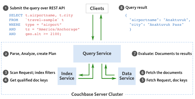
The SELECT statement is executed as a sequence of steps. Each step in the process produces result objects that are then used as inputs in the next step until all steps in the process are complete. While the workflow diagram shows all the possible phases a query goes through before returning a result, the clauses and predicates in a query decide the phases and the number of times that the query goes through. For example, sort phase can be skipped when there is no ORDER BY clause in the query; scan-fetch-join phase will execute multiple times for correlated subqueries.

The following diagram shows the possible elements and operations during query execution.

Figure 2. Query Execution Phases

Some phases are done serially while others are done in parallel, as specified by their parent operator.

The below table summarizes all the Query Phases that might be used in an Execution Plan:

Query Phase	Description
Parse	Analyzes the query and available access path options for each keyspace in the query to create a query plan and execution infrastructure.
Plan	Selects the access path, determines the Join order, determines the type of Joins, and then creates the infrastructure needed to execute the plan.
Scan	Scans the data from the Index Service.
Fetch	Fetches the data from the Data Service.
Join	Joins the data from the Data Service.
Filter	Filters the result objects by specifying conditions in the WHERE clause.
Pre-Aggregate	Internal set of tools to prepare the Aggregate phase.
Aggregate	Performs the COUNT, DISTINCT, SUM, AVERAGE, and other aggregating functions.
Sort	Orders and sorts items in the resultset in the order specified by the ORDER BY clause
Offset	Skips the first n items in the result object as specified by the OFFSET clause.
Limit	Limits the number of results returned using the LIMIT clause.
Project	Receives only the fields needed for final displaying to the user.

Query Phase

Description

Parse

Analyzes the query and available access path options for each keyspace in the query to create a query plan and execution infrastructure.

Plan

Selects the access path, determines the Join order, determines the type of Joins, and then creates the infrastructure needed to execute the plan.

Scan

Scans the data from the Index Service.

Fetch

Fetches the data from the Data Service.

Join

Joins the data from the Data Service.

Filter

Filters the result objects by specifying conditions in the WHERE clause.

Pre-Aggregate

Internal set of tools to prepare the Aggregate phase.

Aggregate

Performs the COUNT, DISTINCT, SUM, AVERAGE, and other aggregating functions.

Sort

Orders and sorts items in the resultset in the order specified by the ORDER BY clause

Offset

Skips the first n items in the result object as specified by the OFFSET clause.

Limit

Limits the number of results returned using the LIMIT clause.

Project

Receives only the fields needed for final displaying to the user.

The possible elements and operations in a query include:

Specifying the keyspace that is queried.
Specifying the document keys or using indexes to access the documents.
Fetching the data from the data service.
Filtering the result objects by specifying conditions in the WHERE clause.
Removing duplicate result objects from the resultset by using the DISTINCT clause.
Grouping and aggregating the result objects.
Ordering (sorting) items in the resultset in the order specified by the ORDER BY expression list.
Skipping the first n items in the result object as specified by the OFFSET clause.
Limiting the number of results returned using the LIMIT clause.

Data Processing Capabilities

Filtering

You can filter the query results using the WHERE clause. Consider the following example which queries for all airports in the America/Anchorage timezone that are at an altitude of 2000ft or more. The WHERE clause specifies the conditions that must be satisfied by the documents to be included in the resultset, and the resultset is returned as an array of airports that satisfy the condition.

The keys in the result object are ordered alphabetically at each level.

Query

SELECT *
FROM   `travel-sample`
WHERE  type = "airport"
       AND tz = "America/Anchorage"
       AND geo.alt >= 2000;

Result

[
   {
      "travel-sample": {
         "airportname": "Anaktuvuk Pass Airport",
         "city": "Anaktuvuk Pass",
         "country": "United States",
         "faa": "AKP",
         "geo": {
            "alt": 2103,
            "lat": 68.1336,
            "lon": -151.743
         },
         "icao": "PAKP",
         "id": 6712,
         "type": "airport",
         "tz": "America/Anchorage"
      }
   },
   {
      "travel-sample": {
         "airportname": "Arctic Village Airport",
         "city": "Arctic Village",
         "country": "United States",
         "faa": "ARC",
         "geo": {
            "alt": 2092,
            "lat": 68.1147,
            "lon": -145.579
         },
         "icao": "PARC",
         "id": 6729,
         "type": "airport",
         "tz": "America/Anchorage"
      }
   }
]

Querying Across Relationships

You can use the SELECT statement to query across relationships using the JOIN clause or subqueries.

JOIN Clause

Before we delve into examples, let’s take a look at the data model of the travel-sample keyspace, which is used in the following examples. For more details about the data model, see java-sdk::sample-application.adoc#datamodel.

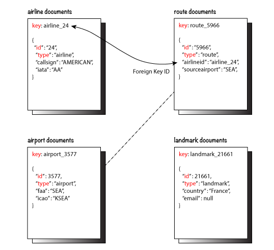Figure 3. Data model of travel-sample keyspace

The first example (Example 1) uses a JOIN clause to find the distinct airline details which have routes that start from SFO. This example JOINS the document of type "route" with documents of type "airline" using the KEY "airlineid".

Documents of type "route" are on the left side of JOIN, and documents of type "airline" are on the right side of JOIN.

The documents of type "route" (on the left) contain the foreign key "airlineid" of documents of type "airline" (on the right).

Example 1: Query

SELECT DISTINCT airline.name, airline.callsign, route.destinationairport, route.stops, route.airline
FROM `travel-sample` route
  JOIN `travel-sample` airline
  ON KEYS route.airlineid
WHERE route.type = "route"
  AND airline.type = "airline"
  AND route.sourceairport = "SFO"
LIMIT 2;

Example 1: Results

[
   {
      "airline": "SY",
      "callsign": "SUN COUNTRY",
      "destinationairport": "MSP",
      "name": "Sun Country Airlines",
      "stops": 0
   },
   {
      "airline": "UA",
      "callsign": "UNITED",
      "destinationairport": "IND",
      "name": "United Airlines",

      "stops": 0
   }
]

Let’s consider another example (Example 2) which finds the number of distinct airports where AA has routes. In this example:

Documents of type "airline" are on the left side of JOIN, and documents of type "route" are on the right side.
The WHERE clause predicate airline.iata = "AA" is on the right side keyspace "airlines".

This example illustrates a special kind of JOIN where the documents on the right side of JOIN contain the foreign key reference to the documents on the left side. Such JOINs are referred to as index JOIN. For details, see Lookup JOIN Clause.

+ Index JOIN requires a special inverse index route_airlineid on the JOIN key ‘route.airlineid’. Create this index using the following command:

CREATE INDEX route_airlineid ON `travel-sample`(airlineid)
WHERE type = "route";

+ Now we can execute the following query.

+ .Example 2: Query

SELECT Count(DISTINCT route.sourceairport) AS distinctairports1
FROM `travel-sample` airline
  JOIN `travel-sample` route
  ON KEY route.airlineid FOR airline
WHERE  route.type = "route"
  AND    airline.type = "airline"
  AND    airline.iata = "AA";

+ .Example 2: Results

[
   {
      "distinctairports1": 429
   }
]

+ Subqueries

+ A subquery is an expression that is evaluated by executing an inner SELECT query. Subqueries can be used in most places where you can use an expression such as projections, FROM clauses, and WHERE clauses.

+ A subquery is executed once for every input document to the outer statement and it returns an array every time it is evaluated. See Subqueries for more details.

+ .Query

SELECT *
FROM   (SELECT t.airportname
        FROM   (SELECT *
                FROM   `travel-sample` t
                WHERE  type = "airport"
                       AND country = "United States"
                LIMIT  1) AS s1) AS s2;

+ .Results

[
   {
      "s2": {
         "airportname": "Barter Island Lrrs"
      }
   }
]

Deep Traversal for Nested Documents

When querying a bucket with nested documents, SELECT provides an easy way to traverse deep nested documents using the dot notation and NEST and UNNEST clauses.

The following query looks for the schedule, and accesses the flight id for destinationaiport=ALG. Since a given flight has multiple schedules, attribute "schedule" is an array containing all schedules for the specified flight. You can access the individual array elements using the array indexes. For brevity, we’re limiting the number of results in the query to 1.

Query

SELECT t.schedule[0].flight AS flightid
FROM `travel-sample` t
WHERE type="route"
  AND destinationairport="ALG"
LIMIT 1;

Results

[
   {
      "flightid": "AH631"

   }
]

NEST and UNNEST

Note that, an array is created with the matching nested documents. In this example:

The ‘airline’ field in the result is an array of the travel-sample documents that are matched with the key route.airlineid.
Hence, the projection is accessed as airline[0] to pick the first element of the array.

Query

SELECT DISTINCT route.sourceairport,
                route.airlineid,
                airline[0].callsign
FROM `travel-sample` route NEST `travel-sample` airline
  ON KEYS route.airlineid
WHERE route.type = "route"
  AND route.airline = "AA"
LIMIT 4;

+ .Results

[
   {
      "airlineid": "airline_24",
      "callsign": "AMERICAN",
      "sourceairport": "ITH"
   },
   {
      "airlineid": "airline_24",
      "callsign": "AMERICAN",
      "sourceairport": "WAW"
   },
   {
      "airlineid": "airline_24",
      "callsign": "AMERICAN",
      "sourceairport": "BKK"
   },
   {
      "airlineid": "airline_24",
      "callsign": "AMERICAN",
      "sourceairport": "GGT"
   }
]

+ The following example uses the UNNEST clause to retrieve the author names from the reviews object.

+ .Query

SELECT r.author
FROM `travel-sample` t UNNEST t.reviews r
WHERE t.type = "hotel"
LIMIT 4;

+ .Results

[
   {
      "author": "Ozella Sipes"
   },
   {
      "author": "Barton Marks"
   },
   {
      "author": "Blaise O'Connell IV"
   },
   {
      "author": "Nedra Cronin"
   }
]

Aggregation

As part of a single SELECT statement, you can also perform aggregation using the SUM, COUNT, AVG, MIN, MAX, or ARRAY AVG functions.

The following example counts the total number of flights to SFO:

Query

SELECT count(schedule[*]) AS totalflights
FROM `travel-sample` t
WHERE type="route"
  AND destinationairport="SFO";

Results

[
   {
      "totalFlights": 250
   }
]

Combining Resultsets Using Operators

You can combine the result sets using the UNION or INTERSECT operators.

Consider the following example which looks for the first schedule for flights to "SFO" and "BOS":

Query

(SELECT t.schedule[0]
 FROM `travel-sample` t
 WHERE type = "route"
   AND destinationairport = "SFO"
 LIMIT  1)
UNION ALL
(SELECT t.schedule[0]
 FROM `travel-sample` t
 WHERE type = "route"
   AND destinationairport = "BOS"
 LIMIT  1);

Results

[
   {
      "$1": {
         "day": 0,
         "flight": "AM982",
         "utc": "09:11:00"
      }
   },
   {
      "$1": {
         "day": 0,
         "flight": "AI339",
         "utc": "23:05:00"
      }
   }
]

Grouping, Sorting, and Limiting Results

You can perform further processing on the data in your result set before the final projection is generated. You can group data using the GROUP BY clause, sort data using the ORDER BY clause, and you can limit the number of results included in the result set using the LIMIT clause.

The following example looks for the number of airports at an altitude of 5000 ft or higher and groups the results by country and timezone. It then sorts the results by country names and timezones (ascending order by default).

Query

SELECT COUNT(*)  AS count,
       t.country AS country,
       t.tz AS timezone
FROM `travel-sample` t
WHERE type = "airport"
  AND geo.alt >= 5000
GROUP BY t.country, t.tz
ORDER BY t.country, t.tz;

Results

[
   {
      "count": 2,
      "country": "France",
      "timezone": "Europe/Paris"
   },
   {
      "count": 57,
      "country": "United States",
      "timezone": "America/Denver"
   },
   {
      "count": 7,
      "country": "United States",
      "timezone": "America/Los_Angeles"
   },
   {
      "count": 4,
      "country": "United States",
      "timezone": "America/Phoenix"
   },
   {
      "count": 1,
      "country": "United States",
      "timezone": "Pacific/Honolulu"
   }
]