Query Workbench

The Query Workbench provides a rich graphical user interface to perform query development.

Using the Query Workbench, you can conveniently explore data, create, edit, run, and save N1QL queries, view and save query results, and explore the document structures in a bucket - all in a single window.

Features of the Query Workbench include:

A single, integrated visual interface to perform query development and testing.
Easy viewing and editing of complex queries by providing features such as multi-line formatting, copy-and-paste, syntax coloring, auto completion of N1QL keywords and bucket and field names, and easy cursor movement.
View the structure of the documents in a bucket by using the N1QL INFER command. You no longer have to select the documents at random and guess the structure of the document.
Display query results in multiple formats: JSON, table, and tree. You can also save the query results to a file on disk.

From the Couchbase Web Console > select the Query menu. By default, the Query Workbench tab is displayed.

The Query Workbench only runs on nodes which are running the Query service. If the Query service is not running on the current node, it provides a link to the nodes in the cluster which are running the Query service.

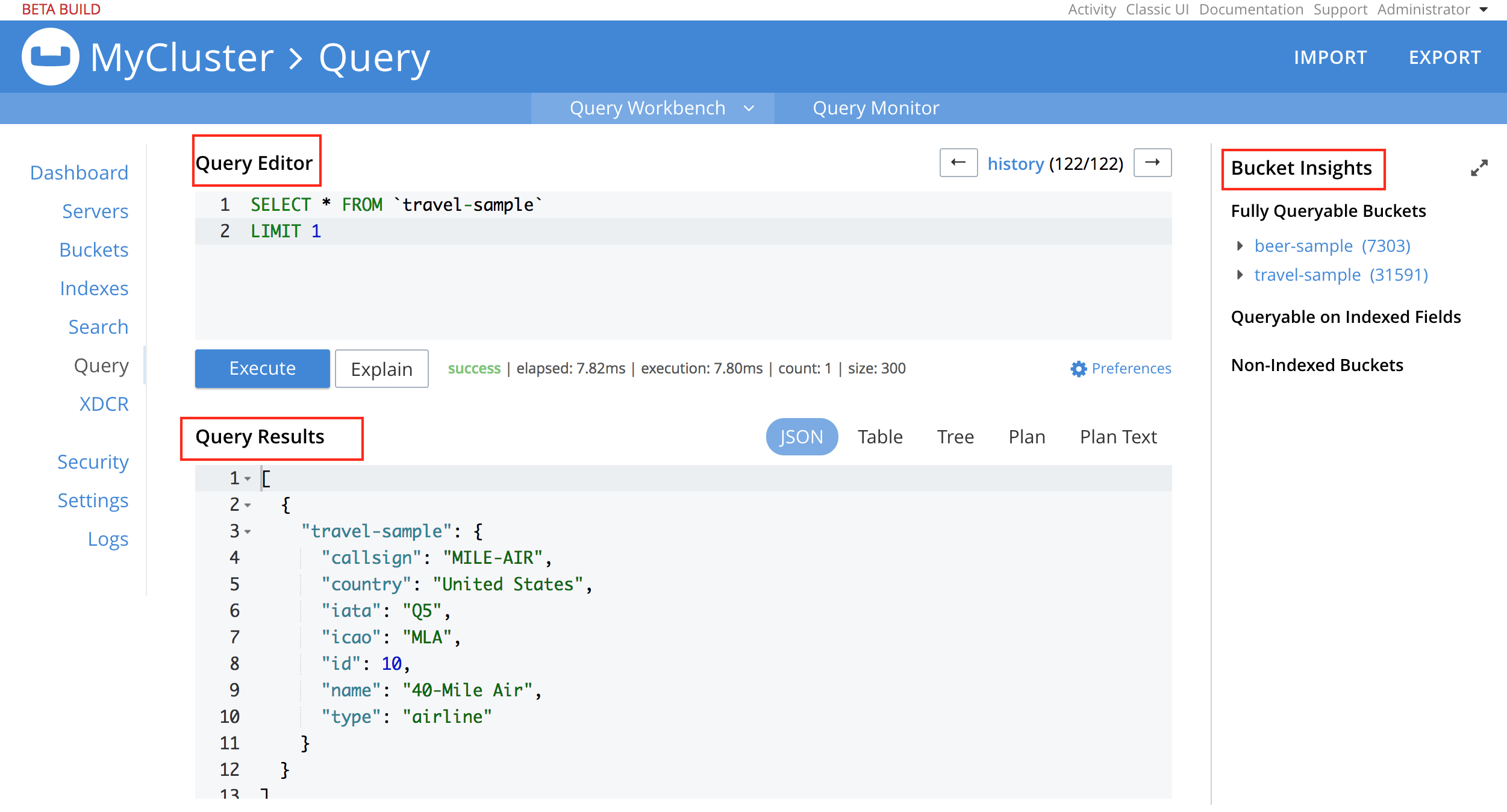
The Query Workbench consists of three working areas as shown in the following figure:

Query Editor
Bucket Insights
Query Results and Plans

Figure 1. Query Workbench Areas

Using the Query Editor

The Query Editor is where you build queries, and run the queries using the Execute button.

You can also execute queries by typing a semi-colon (;) at the end of the query and hitting Enter.

The Query Editor provides the following additional features:

Syntax coloring - For easy viewing, N1QL keywords, numbers and string literals are differently colored.
Auto-completion - When entering a keyword in the Query editor, if you enter the tab key or Ctrl+Space, the tool offers a list of matching N1QL keywords and bucket names that are close to what you have typed so far. For names that have a space or a hyphen (-), the auto-complete option includes back quotes around the name. If you expand a bucket in the Data Bucket Analysis, the tool learns and includes the field names from the schema of the expanded bucket.
Support for N1QL INFER statements - In the Enterprise Edition, the tool supports the N1QL INFER statement.

Run a Query

After entering a query, you can execute the query by either typing ‘;’ and pressing Enter, or by clicking the Execute button. When the query is running, the Execute button changes to Cancel that allows you to cancel the running query. When you cancel a running query, it stops the activity on the server side as well. After running the query, you can use the Explain link to view the execution plan for the query that is executed in the Query Results pane.

The Cancel button does not cancel index creation statements. The index creation continues on the server side even though it appears to have been canceled from the Query Workbench.

View Query History

The tool maintains a history of all the queries executed. Use the arrow keys at the top of the editor to navigate through the history. If you edit a previous query and execute it, the new query is stored at the end of the history. The history is persistent across browser sessions. The query history only saves queries; due to limited browser storage it does not save query results. Thus, when you restart the browser or reload the page, you can see your old queries, but you must re-execute the queries if you want to see their results.

Clearing the browser history clears the history maintained by the Query Editor as well.

Click the history link, at the top of the editor, to open the Query History window. When the window opens, the current query is selected.

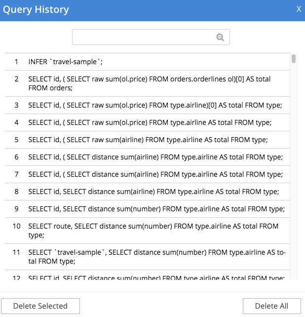
You can scroll through the entire query history, and click to select an individual query to be at the current spot in the history.

Search history - You can search the query history by entering a text in the search box located on the top. All matching queries are displayed. If no matching query is found, then the entire history is displayed.
Delete a specific entry - Click Delete Selected to delete the currently selected query from the history.
Delete all entries - Click Delete All to delete the entire query history.

History Status

The currently shown position in the history is indicated by the numbers next to the history link. For example, (151/152) indicates that query #151 is currently shown, out of a total history length of 152 queries. Use the forward or back buttons to move to the next or previous query in the history. The forward button can also create a new blank query when you are already at the end of the query history.

Import Query

You can load a query from a file into the Query Editor. Click Import and then select a local file that you wish to import. Alternatively, you can drag and drop the file from the Desktop into the Query Editor to a load a file. The content of the file is added in the Query Editor as a new query at the end of the history.

Export Query or Results

You can export the query results or query statement. Click Export to display Export Query / Data window.

Choose the Query Results option to export the results in the JSON file format. Specify the name of the JSON file where results are saved, click Save.
Choose the Query Statement option to export the statement in the .txt format. By default, the query is saved as a text file (.txt) in the Downloads directory when using Firefox and Chrome browsers.

When using Safari, clicking Save loads the data into a new window. You have to save the file manually using the File > Save As menu.

Query Preferences

You can specify the query settings by clicking the query workbench settings button. The Run-Time Preferences window is displayed.

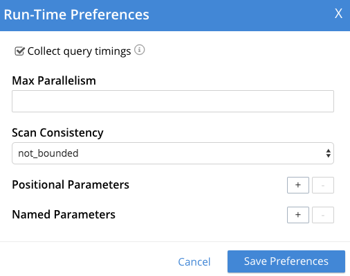
Define the following options and click Save Preferences.

Option	Description
Collect query timings	The server records the timing for most operations in the query plan, showing the updated query plan with the query result. Both graphical and textual query plans are updated with the timing information when the query is complete.
Max Parallelism	This is a cbq-engine option. If you do not specify, the cbq-engine uses its default value.
Scan Consistency	This is a cbq-engine option. Select one of the following options: not_bounded request_plus statement_plus For more information, see N1QL REST API.
Positional Parameters	For the prepared queries, this option allows you to specify values for $0, $1, and so on up to as many positional parameters as you have. Click the + button to add new positional parameters, and the - button to remove the parameters. The parameters are automatically labelled as "$0", "$1", and so on.
Named Parameters	For the prepared queries, this option allows you to specify any number of named parameters. Named parameters must start with the dollar sign ($) for use in prepared queries. Otherwise, they are interpreted as parameters to the Query REST API.

Option

Description

Collect query timings

The server records the timing for most operations in the query plan, showing the updated query plan with the query result. Both graphical and textual query plans are updated with the timing information when the query is complete.

Max Parallelism

This is a cbq-engine option. If you do not specify, the cbq-engine uses its default value.

Scan Consistency

This is a cbq-engine option. Select one of the following options:

not_bounded
request_plus
statement_plus

For more information, see N1QL REST API.

Positional Parameters

For the prepared queries, this option allows you to specify values for $0, $1, and so on up to as many positional parameters as you have. Click the + button to add new positional parameters, and the - button to remove the parameters. The parameters are automatically labelled as "$0", "$1", and so on.

Named Parameters

For the prepared queries, this option allows you to specify any number of named parameters. Named parameters must start with the dollar sign ($) for use in prepared queries. Otherwise, they are interpreted as parameters to the Query REST API.

Viewing the Bucket Insights

The Bucket Insights area displays all installed buckets in the cluster. By default, when the Query Workbench is first loaded, it retrieves a list of available buckets from the cluster. The Bucket Insights pane is automatically refreshed when buckets or indexes are added or removed.

Click the Resize button query workbench bucket resize to enlarge the Bucket Insights pane, the Query Editor and Query Results areas are resized accordingly.

The buckets are grouped into the following categories based on the indexes created for the bucket:

Fully Queryable Buckets: Contain a primary index or a primary index and secondary indexes.
Queryable on Indexed Fields: Do not contain a primary index, but have one or more secondary indexes.
Non-Indexed Buckets: Do not contain any indexes. These buckets do not support queries. You must first define an index before querying these buckets.

With the Enterprise Edition, you can expand any bucket to view the schema for that bucket: field names, types, and if you hover the mouse pointer over a field name, you can see example values for that field. Bucket analysis is based on the N1QL INFER statement, which you can run manually to get more detailed results. This command infers a schema for a bucket by examining a random sample of documents. Because the command is based on a random sample, the results may vary slightly from run to run. The default sample size is 1000 documents. The syntax of the command is:

INFER bucket-name [ WITH options ];

where options is a JSON object, specifying values for one or more of sample_size, similarity_metric, num_sample_values, or dictionary_threshold.

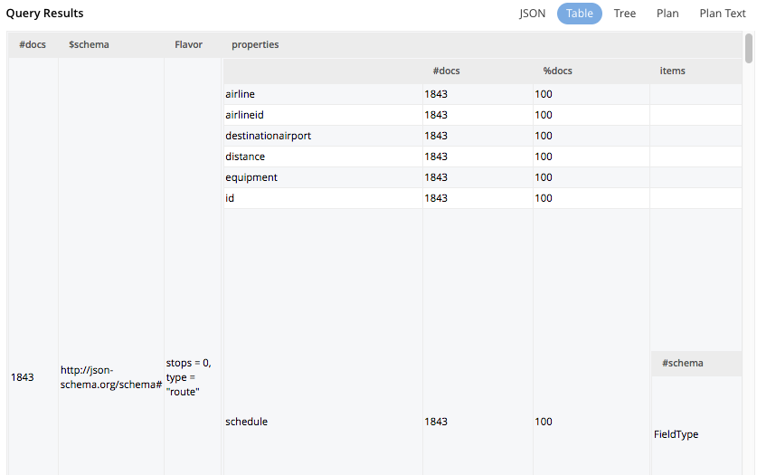
Figure 2. Sample INFER statement: INFER travel-sample with {"sample_size": 3000};

Viewing the Query Results

When you execute a query, the results are displayed in the Query Results area. Since large result sets can take a long time to display, we recommend using the LIMIT clause as part of your query when appropriate.

When a query finishes, the query metrics for that query are displayed on the right side of the Execute and Explain buttons.

Status - Shows the status of the query. The values can be: success, failed, or HTTP codes.
Elapsed - Shows the overall query time.
Execution -Shows the query execution time.
Result Count - Shows the number of returned documents.
Mutation Count - Shows the number of documents deleted or changed by the query. This appears only for UPDATE and DELETE queries instead of Result Count. Result Size: Shows the size in bytes of the query result.

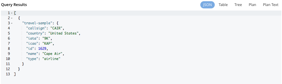
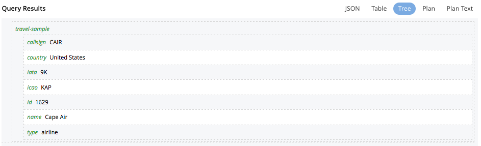
The following figures display the result of the query SELECT * FROM `travel-sample` LIMIT 1; in different formats.

You can choose to view the results in one of the following formats:

JSON Format: JSON, where the results are formatted to make the data easy to read. You can also expand and collapse objects and array values using the small arrow icons next to the line numbers.
Table Format: Table, where the results are presented in a tabular format. The tool converts the JSON documents to HTML tables, and presents sub-objects or sub-arrays as sub-tables. This format works well for queries that return an array of objects, like select `beer-sample`.* from `beer-sample`;. You can hover the mouse pointer over a data value to see the path to that value in a tool tip. You can sort a column by clicking the column header.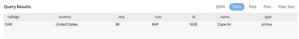
Tree Format: Tree (or list), where the results are presented in a tree (or list or outline) format. Each sub-object or sub-array is displayed as a sub-list. You can hover the mouse pointer over a data value to see the path to that value in a tool tip.

Query Plans

Each time a query is executed, an explain command is automatically run in the background to retrieve the query plan for that query. You may also generate the query plan by clicking the Explain link. This query plan may be shown as either:

Plan

This is where the results are presented in a graphical format.

At the top, it shows a summary which also shows lists of the buckets, indexes, and fields used by the query.

At the bottom is a data-flow diagram of query operators, with the initial scans at the right, and the final output on the left.

Potentially expensive operators are highlighted.

Once the query is complete, if you have selected the Collect query timings option in the preferences dialog, the query plan will be updated with timing information (where available) for each operation.

The data flow generally follows these steps:

Scan
Fetch
Filter
Projection (part 1)
Order
Projection (part 2)

Projection is split into two parts (one before Order and one after Order), but Query Workbench shows only the first part.

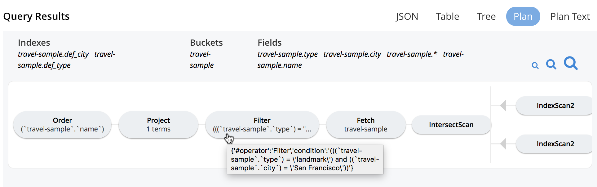
+ Hovering over any unit of the plan shows more details of it. In this example query:

Unit name Information shown when hovered over

Unit name	Information shown when hovered over
Order	{'#operator':'Order':'sort_terms': [{'expr':'(`travel-sample`.`name`)'}]}
Project	{'#operator':'InitialProject':'result_terms': [{'expr':'self','star':true}]}
Filter	{'#operator':'Filter','condition':'(`travel-sample`.`type`) = \'landmark\') and ((`travel-sample`.`city`) = \'San Francisco\''}
Fetch	{'#operator':'Fetch','keyspace':'travel-sample','namespace':'default'}
IntersectScan	(none)
IndexScan2 (above)	{'#operator':'IndexScan2','index':'def_city','index_id':'d51323973a9c8458','index_projection': {'primary_key':true},'keyspace':'travel-sample','namespace':'default','spans': [{'exact':true,'range':[{'high':'\San Francisco\'','inclusion':3,'low':'\'San Francisco\''}]}],'using':'gsi'}
IndexScan2 (below)	{'#operator':'IndexScan2','index':'def_city','index_id':'a11b1af8651888cf','index_projection': {'primary_key':true},'keyspace':'travel-sample','namespace':'default','spans': [{'exact':true,'range':[{'high':'\'landmark'\'','inclusion':3,'low':'\'landmark\''}]}],'using':'gsi'}

Order

{'#operator':'Order':'sort_terms':

[{'expr':'(travel-sample.name)'}]}

Project

{'#operator':'InitialProject':'result_terms':

[{'expr':'self','star':true}]}

Filter

{'#operator':'Filter','condition':'(travel-sample.type) = \'landmark\') and ((travel-sample.city) = \'San Francisco\''}

Fetch

{'#operator':'Fetch','keyspace':'travel-sample','namespace':'default'}

IntersectScan

(none)

IndexScan2 (above)

{'#operator':'IndexScan2','index':'def_city','index_id':'d51323973a9c8458','index_projection':

{'primary_key':true},'keyspace':'travel-sample','namespace':'default','spans':

[{'exact':true,'range':[{'high':'\San Francisco\'','inclusion':3,'low':'\'San Francisco\''}]}],'using':'gsi'}

IndexScan2 (below)

{'#operator':'IndexScan2','index':'def_city','index_id':'a11b1af8651888cf','index_projection':

{'primary_key':true},'keyspace':'travel-sample','namespace':'default','spans':

[{'exact':true,'range':[{'high':'\'landmark'\'','inclusion':3,'low':'\'landmark\''}]}],'using':'gsi'}

+ In general, the preference of scan is

Covering Index
Index Scan
Intersect Scan
Union Scan, and finally
Fetch

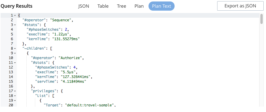
Plan Text

This simply shows the text output of the explain command.